Example usage

To use spenv in a project:

import spenv
import numpy as np
import pandas as pd
import matplotlib.pyplot as plt

print(spenv.__version__)

0.1.1

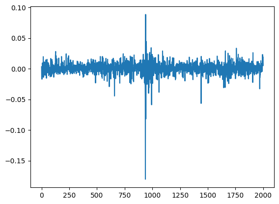
The dataset used in this example is the nyse data from the astsa R package, scraped from the astsadata Python module.

path = "https://raw.githubusercontent.com/evorition/astsadata/main/astsadata/data/nyse.csv"
data = pd.read_csv(path)

plt.plot(data.value)
plt.show()

Spectral Analysis

These functions can be used for spectral estimation of univariate or multivariate time series.

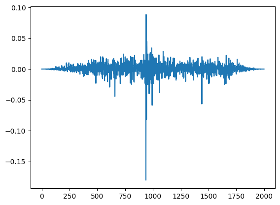
Tapered time series

spec_taper applies taper smoothing to a time series.

plt.plot(spenv.spec_taper(data.value, p=0.25))
plt.show()

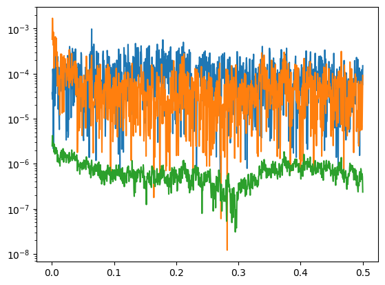
Multivariate Periodogram

In this example, the (x, |x|, x²) set is used to generate a matrix for multivariate spectral estimation.

# reshape to a 2D array
vec = data['value'].values.reshape((-1,1))

# generate matrix
mat = np.concatenate([vec, np.abs(vec), vec**2], axis=1)

# estimate
pgram = spenv.mvspec(mat)

plt.plot(pgram['freq'], pgram['spec'][:,0])
plt.plot(pgram['freq'], pgram['spec'][:,1])
plt.plot(pgram['freq'], pgram['spec'][:,2])
plt.yscale('log')
plt.show()

Spectral Envelope

The specenv function computes the spectral envelope for the time series provided. The spec_opt automatically smoothes a time series based on the approach presented in Time Series Analysis and Its Applications with R Examples.

envelope = pd.DataFrame(spenv.specenv(mat), columns= ['freq', 'specenv', 'b1', 'b2', 'b3'])
envelope.head(10)
# the first and second variables show the frequencies and the envelope estimated
# the remaining columns show the coefficients

/home/docs/checkouts/readthedocs.org/user_builds/spenv/checkouts/latest/src/spenv.py:322: ComplexWarning: Casting complex values to real discards the imaginary part
  specenv[k] = ev[0]
/home/docs/checkouts/readthedocs.org/user_builds/spenv/checkouts/latest/src/spenv.py:324: ComplexWarning: Casting complex values to real discards the imaginary part
  beta[k, ] = b/np.sqrt(np.sum(b**2))

	freq	specenv	b1	b2	b3
0	0.0005	0.011437	-0.068884	-0.633744	0.770470
1	0.0010	0.026382	0.004831	-0.233153	0.972428
2	0.0015	0.016049	-0.023791	0.270289	-0.962485
3	0.0020	0.006597	0.043528	-0.209931	0.976747
4	0.0025	0.015982	-0.044775	-0.391717	0.918996
5	0.0030	0.004889	-0.081479	0.398915	-0.913361
6	0.0035	0.003250	-0.054930	0.156253	0.986189
7	0.0040	0.002765	0.278932	0.116058	-0.953272
8	0.0045	0.000000	-0.130564	-0.091072	0.987248
9	0.0050	0.004344	-0.096177	-0.152392	-0.983629

# plot the spectral envelope
plt.plot(envelope['freq'], envelope['specenv'])
plt.show()

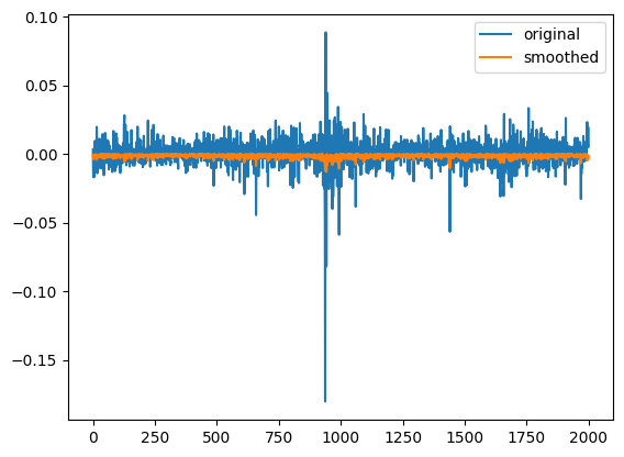
# time series smoothing
smoothed = spenv.spec_opt(vec, np.abs, np.square)
# create a dataframe from the original and smoothed data
result = pd.DataFrame({'original': vec.flatten(), 'smoothed': smoothed})

/home/docs/checkouts/readthedocs.org/user_builds/spenv/checkouts/latest/src/spenv.py:322: ComplexWarning: Casting complex values to real discards the imaginary part
  specenv[k] = ev[0]
/home/docs/checkouts/readthedocs.org/user_builds/spenv/checkouts/latest/src/spenv.py:324: ComplexWarning: Casting complex values to real discards the imaginary part
  beta[k, ] = b/np.sqrt(np.sum(b**2))

for col in result.columns:
    result[col].plot(legend=True)
plt.show

<function matplotlib.pyplot.show(close=None, block=None)>